Controlling the drawdowns.
For instance, we have a maximal set drawdown in % of the capital. The method involves equaling the starting risk for the position to a fixed fraction of the set maximal drawdown:
Num_Lots = % Risk * (Capital – (1 – Max_%_Drawdown) * Maximal_Capital) / starting_risk_per_unit_assets / 100
If our current capital is $100 000, maximal reached capital $110 000 and maximal allowable drawdown 20%, we can risk a sum equal to 10% of the drawdown. Then our risk would be $1200 (10% * ($ 100 000 – 80% * $110 000)). Thus, if the risk per share is $0.1, we can buy 120 lots of 100 shares. If price changes were uninterrupted, transaction costs negligible, odd lots permitted and the traders’ timing perfect, then this method would guarantee tha drawdown never goes over the limit .
Another option of drawdown control is taking into account its maximal historical value (with a fair reserve):
Num_contracts = Capital / (2 * Max_Drawdown + margin_per_contract)
Kelly’s method.
This method defines the optimal percent of risk that should be employed to maximalise the “usefulness” function presented as logarithm of the capital. Relatively to gambling and further, to stock trading was developed by professor Edward Thorpe3.
In the trading game of doctors of sciences described in the previous article (where 60% of cases won and 40% lost the bet), the optimal bet according to Kelly is 20% of current capital. From Table 3 of that article we can see that the 50-percentile k-50 really reaches its maximum of 7940 when the stake is 20%. What’s not so smooth-looking is that 50% of drawdowns are over 79.09$ and the maximal drawdown reaches 99.43%. Are we willing to reach the maximal possible profit at the cost of losing 99% of the capital somewhere along the way? If we want to break the record of Larry Williams, then maybe so. As Ralph Vince explained that achievement: “He is one of the few persons really able to trade with fully optimal values and pass through the concomitant drawdowns” .
Kelly’ s method defines the percent of risk as:
Kelly%=%win – %loss * Avg_profit / Avg_loss
Hence we can estimate the position size:
Num_Lots = Kelly% * Capital / starting_risk_per_unity_of_assets
Thorpe recommends using % of risk within 0.5 * Kelly <= % risk < Kelly bounds. Table 1 shows the results that allow us to conclude that with risks 18% of Kelly and more our simple trading system is no longer profitable.
| Table1. Results of testing Kelly’s method. | ||||||||||||||||||||||||||||||||||||||||||||||||||||||
|
Optimal f.
This method of estimating the optimal % of risk has been improved by Raplh Vince. While Kelly’s formula use only average values from past trades, Raplh Vince proposed to take into account all trades, solving the task of optimization of the relative end capital TWR as a function of f.
We take the negative value of the loss, hence the minus. Actually, this method implies that in the future the trade results will be about the same, but possibly in another order. Solving the TWR maximization, we find the f = fopt value, where the TWR function reaches its maximum. From fopt we define position size:
Number_Lots = fopt * Capital / ( - Max_Loss)
A simple method of calculation is presented in Appendix2. According to it the maximal drawdown with optimal f value will be at least fopt % of account. I.e. if our fopt is, say, 0.5, then our drawdowns will reach at least 50%. Raplh Vince says that: ”if you are not trading for optimal profits, then you belong in an asylum, not in the market” . Still, he does not consider the fact that a 99% drawdown when trading for an “optimal profit” can land us in asulym – or at least in hospital after trying to explain to the family or investors. It doesn’t help that the capital grows on then.
Besides, the distribution of trade results has a most profound influence on the fopt value. So fopt values for two strategies that in the end bring the same profit and have the same maximal loss may be very different.
The weak spot of the optimal f method is that it is fully based on the system’s historical results, on maximal loss to be exact. The risk level set when using fopt, means we‘ll never have a larger loss.
Unlike gambling, where the outcomes are known and probabilities constant, in trading we have a multitude of random outcomes with undetermined probability of winning. The maximal loss is a nondescreasing step function, with random amplitude leaps occurring at random moments.
So, there is no real evidence to suppose that the maximal loss and maximal drawdown achieved will persist in the future. To calculate fopt it is possible to use in the TWR formula, instead of the maximal loss a value:
Max_Loss_Evaluation = Avg_Loss – 3.5 Standart_Deviation_of_Loss
But this doesn’t solve the problem yet. The outcome of a future trade is evidently random, so then the optimal f for is must also be random. The fopt value calculated from previous trades won't be really optimal for future trades, unless we turn to really reckless trading. Let's show an example of this.
We calculate the optimal f for a model system (num = 1) for several trades in a row, as shown in Appendix1. For the last 10 trades the optimal values would be 0.135, 0.134, 0.131, 0.123, 0.156, 0.142, 0.149, 0.137, 0.155, 0.165. So before the last trade we choose a value of f equal to 0.155 while the optimal value would be 0.165 – we take a less-than-optimal risk. Even worse, the third trade from the right has an optimal f of 0.137, while we consider it to be 0.149, accepting too much risk. So the so-called optimal f is really far from optimal.
The Safe f.
Leo Zamansky and David Stendahl tried to overcome large drawdowns by adding a special limit of maximall allowable drawdown.
Max_Drawdown <= Max_Allowed_Drawdown
Another way is to use the maximal drawdown or its estimate instead of the maximal loss in the TWR formula for calculations the safe f.
Optimal f with volatility.
Murray Ruggiero proposed to adapt the position size calculated using the optimal f to the current market volatility. . This is founded on the hypothesis that when the market volatility is low, the chance of having a large loss is larger than when the volatility is high. We normalize the volatility from 1 to 0, where 0 is maximal volatility, and 1 – minimal:
Volatilitynorm = (Max_Volatility – Current_Volatility / (Max_Volatility – Min_Volatility)
Then Num_Lots = fopt * Volatilitynorm * Capital / ( -Max_Loss_Estimate)
Here the, fopt is calculated also using the maximal loss evaluation.
Fixed Ratio.
A common problem of all methods using a fixed fraction of the capital is that different methods either maximize the capital growth without relation to risk (i.e. the optimal f) or minimize the risk (i.e. risking not more than x% of capital). Trying to solve this conflict Ryan Jones concludes that the relation of the number of lots traded to capital growth needed to increase the number of lots by one (or the minimal increment) should be a constant:
Previous_Capital+Num_Lots * Delta = Next_Capital
Where Delta defines how aggressive or conservatiove is our application of money management: the more Delta, the larger profit per lot need we receive to increase the number of lots traded. The author proposes using as Delta a part of the maximal drawdown. Our experiments show it’s much better to use volatility.
Table2 lists the results of testing a basic system with the Jones’ algorithm and Delta proportional to volatility. The method is unprofitable with small Delta values, then leaps to maximal profits, after which both profit and maximal drawdown monotonously decrease as Delta grows.
| Table2. The results of testing the fixed ratio method. | ||||||||||||||||||||||||||||||||||||||||||||||||||||||
|
The idea behind this method looks quite doubtful: increasing the number of lots traded from one to two is not equivalent to increasing the number from 10 to 11 (as states Ryan Jones), and an increase from 10 to 20 is a 100% increase. The trader is concerned not about the quantity of contracts, but capital growth and risk in relative values.
Let us perform some manipulations according to Ryan Jones. With a few mathematical transformations (see Appendix3) we make an expression:
Num_Lots = 0.5 + (2 * Profit/Delta + 0.25)^(0.5)
So the number of lots in fixed ratio trading is proportional to the square root of the capital. All variants of fixed ratio trading define the number of lots traded as depending on the capital linearly. Anyone familiar with the basics of mathematical analysis know that at low X values
y = a * x^(0.5) is larger than the linear y = a * x, and vice versa at high X values (see Ill. 1). Hence with a small capital the fixed relation method prescribes trading a larger number of lots than the fixed share of capital, and a smaller number of lots with a larger capital . In other words, the fixed ratio method recommends higher risks with small capitals than the so-called “risky methods” criticized. Practically, this “new” method also involves risking a fixed part of the capital, in a more aggressive way compared to the original. The book examples showing the advantages have been skillfully selected so that drawdowns occur only after the capital has grown significantly.
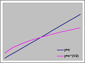
Ill. 1. Comparison of function values with different arguments
As to Ryan Jones’ attempt to break the trading record of Larry Williams in The Robbins 2001 Futures Trading Contest described in the previous article, he failed again... After his account grew by 600% from $15 000 to $107 000, he sent an offer to buy his method, proven by statements capable to bring such profits. Besides, he offered a $299 per month subscription to stay informed of all trades taken in the contest. As a result the drawdown on his capital reached 95%, just what had to be proven.
The method of Larry Williams.
During his record-breaking trading Larry Williams used the Kelly’s formula where the starting risk was defined by the size of the margin per futures fontract. The dynamics of the capital were also noteworthy: first a growth from $10 000 to $210000, then dropped to $700 000 (67% drawdown) and the year was finished at $1100000. By the way, Ralph Wince was working for Williams as programmer. Now Larry Williams recommends the following varian of the fixed fraction method:
Num_Lots = % risk * Capital / (- Max_Drawdown) / 100
Playing the “market’s money”. As experience shows, for an investor it is much more important not to lose a small part of the starting capital than to lose a substantial part of the profits. The idea is taking smaller risks on starting capital and larger, more aggressive on profits received:
Num_Lots = (%riskstart_capital) * (Starting_Capital + MinList(Profit, 0)) + %riskprofit * MaxList(Profit, 0)) / starting_risk_per_unit_of_assets / 100
Pyramid building. All the methods described above define the starting risk for opening the position. The current or effective risk of an open position is, actually, different. It may be expressed as:
Effective_Risk = MarketPosition * (Entry_Price – Current_Exit_Price) *
Num_Lots * Price_of_a_Point
where MarketPosition equals 1 for long positoins, -1 for short, 0 for no position. Until the trade has no unrealized (paper) profit, the effective risk is positive. A trade protected by a stop-loss order at breakeven level has zero effective risk. As soon as the stop loss is moved past breakeven level, the effective risk becomes negative – which means the position has a guaranteed profit, protected by the stop loss. The capital is no longer subject to risk, so we can risk the guaranteed profit, increasing the position size correspondingly.
Additional_Number_Lots = % risk_guaranteed_profit * (- MinList(Effective_Risk, 0)) / starting_risk_per_unit_of_assets / 100
Here MinList( ) is the least value from the list. Clearly, we must not take the %risk_guaranted_profit larger than the optimal for the guaranteed profit. A variant of this method where a constant risk is maintained on the basis of guaranteed profits is described by Titov .
Let us now see it all on an example. If we reinvest the guaranteed profits with the same risk, then, as Table3 shows, profits will increase over 4 times and drawdowns 2.8 times. If we increase the risk for guaranteed profits, net profit skyrockets – but unhappily, drawdowns increase even more.
| Table3. Reinvesting the guaranteed profits. | ||||||||||||||||||||||||
|
Regulating the position size on the basis of its risk and volatility. The risk of an open position is usually controlled by exit rules set in the system. For instance, moving stop levels follow the price to increase starting risk or lock down a part of paper profits. But a much more viable idea is to limit the maximal risk and volatility of an open position in relation to the capital. All we need for this is track the values as often as needed.
Excessive_risk = Num_lots * Current_risk_per_unit_of_assets – Max%risk * Capital / 100
and
Excessive_volatility = Num_lots * Current_volatility_of_assets –
Max%volatility * Capital / 100
As soon as any of those becomes positive, we decrease the position size by a value equal to:
Excessive_num_lots = Excessive_risk / Lot_price
Or correspondingly by:
Excessive_number_lots = Excessive volatility / Lot_price
The practical rationale of this methods is closing a part of the position without waiting for the system signal, when the prices move very fast and far, too far and fast for a trailing stop or a closing point to follow. This solves two tasks at once: first, the risk and volatility are supported at set levels, second, positions frequently close at extreme prices with favourable slippage.
Such methods for one strategy on one asset can be easily applied on the TradeStation platform as shown in App.1. But since real trading involves several strategies applied to portfolios of assets, frequently at different time frames but with a common portfolio capital.
| Appendix 1. The Simplest System with Money Management. | ||
|
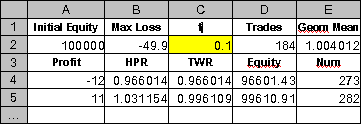
| Appendix 2. Calculating the optimal f in Excel. | ||
|
| Appendix 3. Deriving the formula for the fixed fraction method. | ||
|