A little sidetracking and something on Position sizing
I've been in trading for a long time and don't plan to stuff my pockets with cash and quit tomorrow. So all I am doing in the field of money management is limited to position sizing - and, furthermore, only decreasing the size, no leverage ever. In the extreme case a position may be equal to the limit, but most usual it would be equal to only a part of the funds I assign to trading a particular equity. So to find this optimal size we need to know what maximal adverse drawdown is possible with the given strategy.
Since the same methods of position sizing may (and should) be used in different trading systems, it would be preferable to implement them as separate Easy Language functions called on at due time. As an example I will provide codes for two MM-functions. In one the amount of equity bought is determined by a simple variation of the FixedFractional method (opening a position based on a fixed part of the account), in the other the position size is controlled by volatility. I'd make a reservation at once - definite coding might vary zdepending on the market traded. For instance, these codes are optimized for thrading lots of 100 shares, long trades only, execute on Close price, starting capital = $10.000, profits reinvested, no leverage.
| Appendix 1. This function calculates the number of shares based on fixed fraction of equity per trade. | ||
|
| Appendix 2. This function calculates the number of shares to trade based on risk-volatility model. | ||
|
Now we need to add lines responsible for controlling the number of shares bought on each signal. For the Fixed Fractional strategy add the following:
Inputs: Capital(10000), {Initial capital}
Lot(100), {Minimum shares in 1 Lot}
Fract(50); {Fraction % of equity per trade}
Vars: Num(0);
Num = $MM_Fract(Capital, Lot, Fract);
For the risk/volatility strategy:
Inputs: Capital(10000), {Initial capital}
Lot(100), {Minimum shares in 1 Lot}
LenVolat(14), {Length of average volatility}
Risk(1); {Risk in percent of volatility}
Vars: Num(0);
Num = $MM_Volat(Capital, Lot, LenVolat, Risk);
Correspondingly, the buy commands in the signal codes must be completed with:
... Buy Num Shares at Close;
Please pay attention that in the first case the position is always opened as 50% of the current account (Fract=50), in the second case the position size is determined by 1% of the account for 14-period ATR (Risk=1, LenVolat=14)/ Those values were chosen to provide approximately the same profits form both methods on the same data and with the same strategy. In those cases with both methods of position sizing the average risk per trade is about 2% of the account.
As the "basic" system I've used a simple system based on the price channel breakout indicator (also known as the "Nick Rypock Trailing reverse") on hourly XXX data from January 1998 to July 2001
After adding the links to money management functions to the signal code we have two strategies with the same algorithm of signal acquisition but with different position sizing routines. On comparison the profit values and profit curves for the test period are very similar:
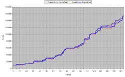
Dark blue line - the Fixed Fractional strategy equity. Blue line- risk/volatility strategy equity.
Yet if we look at a standard Omega strategy report we won't get a comprehensive answer about either position sizing methods. Omega's in-built algorithms allow to analyze only two money management methods - fixed number of contracts and fixed sum of money. As a result, the values fed out appear to be meant for cheating and pacifying the user in regard to possible risks, not for objective evaluation of the possible adverse factors that are bound to pop up somewhere on the road to wealth.
The first thing I felt was missing was the percentile DrawDown expression in percents of the account traded.
Here comes the real DrawDown!
We'll consider a drawdown the result of a series of adverse trades that keeps a new peak from appearing on the equity curve of the trading system. Adverse trades include more than just losing - profitable trades that do not create a new, higher equity value may be included in drawdown periods. Again, we don't care for the absolute value of the drawdown. A drawdown of $10.000 on a $200.000 account will be 5% and hardly a source of distress, but a drawdown of $10.000 on a $20.000 account will probably be far beyond acceptable limits. So our principal goal will be determining the drawdown as a percent of the account current size.
This cannot be achieved in Omega no matter how hard you try - all drawdowns are in absolute values. Something we might use - the UnderWater Equity is calculated in percents, but for some reason only monthly, disrupting the picture completely. There may be a long discussion as to whys and hows, but a bitter answer is evident - the industry of getting naive people to overfit their curves is much, much more profitable compared to stocks trading per se. So we just have to see what can be done.
Luckily Omega can export practically any kind of information to a text file to be processed in other applications. Let's then define what tasks are there to be solved:
· Define the current equity, considering the starting capital and profits from trades.
· Define the peak of the equity curve (top account size) from which we'll calculate the percentile DrawDown.
· Calculate the current percentile DrawDown in a series of adverse trades.
· Calculate the maximal percentile DrawDown for the period.
It would be wise to use an additional Easy Language function to perform all calculations and create a .CSV file that can be later processed in Excel.
| Appendix 3. This function calculates and exports strategy percentage Profits, Equity and DrawDowns. | ||
|
Now add in the end of the strategy code Value10 = $DD_Report(Capital); o have all the data after charting the strategy exported to a file named C:\DD_report.csv.
Probably only two columns here require explanations - the AbsPercProfit is the percentile profit or loss that could be achieved in the trade if all the available funds were fully used. The EqPercProfit is the percentile profit or loss achieved "really" with the position sizing active.
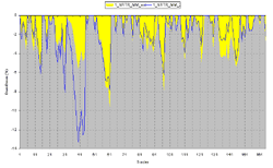
This file may be plotted in Excel in a variety of ways. but it's more interesting to compare the strategy results using different money management techniques. To do so I've placed reports from both systems on separate Excel file sheets and compared them. The equity curves were already shown above, this is what the DrawDowns look like:
Again, I indicate that comparing definite money management methods belongs in a separate study, while here is provided a way to extract from Omega the necessary information for further study. The Excel file those examples were based on can be downloaded here (there is no macros, etc., alltransformations to be performed manually). The data from the DD_report.csv for vever strategy is pasted to separate "Report 1" and "Report 2" sheets. The "Profit 1" and "Profit 2" sheets are used to compare the AbsPercProfit and EqPercProfit values of the strategies, i.e. performance of the capital. The "Profit Compare", "Equity Compare" and "DD Compare" sheets are used to compare, correspondingly, the profits, equity and drawdowns of the money management methods. The ranges of the input data for the plots are to be corrected manually in every separate case.